Matrix calculator with working: determinant, inverse, rank, eigenvalues
Enter a matrix in the table, and the solver computes the determinant three ways, finds the inverse by Gauss–Jordan elimination or through the adjugate, the rank, powers, products and eigenvectors, explaining every step.
determinant [2 1 3; 0 -1 4; 1 2 0]
inverse [2 1; 5 3]
rank [1 2 3; 2 4 6; 1 0 1]
eigenvalues [2 1; 1 2]
[1 1; 1 0]^10
[1 2; 3 4] * [0 1; 1 0]
determinant [1 2 0 3; 0 1 4 0; 2 0 1 1; 1 1 0 2] by cofactor expansion
Loading the solver…
What you can type
Choose an operation (determinant, inverse, rank, eigenvalues, power, product or transpose) and fill in the table. The size changes with the “−” and “+” buttons (up to 6 × 6, and up to 8 × 8 for rank and products); an empty cell counts as zero, and the arrow keys and Enter move between cells. Numbers can be integers, fractions (1/2) or decimals (0.5). You can paste a block of cells from Excel or Google Sheets, lines of text, or something like [[1, 2], [3, 4]] into any cell, and the table adjusts its size.
The same can be written as a line: the matrix in square brackets, rows separated by semicolons, numbers by spaces: “determinant [2 1 3; 0 −1 4; 1 2 0]”, “inverse [2 1; 5 3]”, “[1 1; 1 0]^10”, “[1 2; 3 4] * [5; 6]”. For the determinant you can choose the method: cofactor expansion along a row, Gaussian elimination, or the rule of Sarrus; for the inverse, Gauss–Jordan elimination or the adjugate. All calculations are exact, with fractions.
The determinant: by how much area changes
A $2 \times 2$ matrix describes a transformation of the plane: its columns are where the unit vectors $\mathbf e_1$ and $\mathbf e_2$ end up. The unit square becomes the parallelogram on these two columns, and its area is the absolute value of the determinant. The sign tells you whether the plane has been flipped over, as in a mirror. For a $3 \times 3$ matrix it’s the same with volume: the unit cube becomes the parallelepiped on the three columns. A determinant of zero means the transformation flattens space, and area or volume disappears. Such a matrix is called singular: it has no inverse, and its rows are linearly dependent.
For $3 \times 3$, expanding along the first row opens up into six products of three numbers each, three with a plus and three with a minus. They’re easy to remember with the “rule of triangles”: plus for the main diagonal and the two triangles with a base parallel to it; minus for the same with the other diagonal. The Frenchman Pierre Sarrus suggested copying the first two columns to the right, and then all six products can be read along diagonals. The solver draws this scheme.
For big matrices, cofactor expansion is hopeless: at $n = 10$ it has more than three and a half million terms. Gaussian elimination is much faster. Adding a multiple of one row to another doesn’t change the determinant; swapping two rows changes its sign. These operations bring the matrix to triangular form, and the determinant of a triangular matrix is the product of the numbers on its diagonal. For $10 \times 10$ that’s a few hundred operations.
The inverse matrix
The inverse matrix $A^{-1}$ undoes the transformation: $A \cdot A^{-1} = A^{-1} \cdot A = I$, where $I$ is the identity matrix. It exists exactly when $\det A \ne 0$: flattened space can’t be unfolded again.
Gauss–Jordan elimination. Write $A$ and $I$ side by side, giving the matrix $(A \mid I)$, and use elementary row operations to turn the left half into the identity. Each such operation is multiplication on the left by some simple matrix; together they give a matrix that turns $A$ into $I$, that is, $A^{-1}$. The right half undergoes the same multiplications and turns from $I$ into $A^{-1}$. If some column has no pivot, the matrix is singular.
Why the formula works: in the product $A \cdot \operatorname{adj} A$ the diagonal holds the cofactor expansion of the determinant along a row, that is, $\det A$, and off the diagonal it holds the expansion of the determinant of a matrix with two equal rows, that is, zero. For $2 \times 2$ this is the familiar rule: swap the entries on the main diagonal, change the signs on the other diagonal and divide by the determinant. For big matrices the adjugate needs many minors, and Gaussian elimination wins.
Rank
The rank is the largest number of linearly independent rows of a matrix; it has the same number of independent columns. It’s found by Gaussian elimination: bring the matrix to row echelon form and count the non-zero rows, that is, the pivots. In the matrix $\begin{pmatrix} 1 & 2 & 3 \\ 2 & 4 & 6 \\ 1 & 0 & 1 \end{pmatrix}$ the second row is twice the first; after elimination it becomes zero, and the rank is 2. The rank decides the fate of a system of equations: it is consistent when the rank of the matrix equals the rank of the augmented matrix, and the solution is unique when, in addition, it equals the number of unknowns (the Rouché–Capelli theorem).
Eigenvalues and eigenvectors
Almost every vector gets turned by a matrix. An eigenvector is the exception: it stays on its own line and is only stretched by a factor of $\lambda$, $A\mathbf v = \lambda\mathbf v$. The number $\lambda$ is an eigenvalue. Rewrite the equality as $(A - \lambda I)\mathbf v = 0$: such a homogeneous system has a non-zero solution only when $\det(A - \lambda I) = 0$. This is called the characteristic equation, and its roots are the eigenvalues. For each root, the eigenvectors are found by solving the system with Gaussian elimination.
For $A = \begin{pmatrix} 2 & 1 \\ 1 & 2 \end{pmatrix}$ we get $\det(A - \lambda I) = (2 - \lambda)^2 - 1 = \lambda^2 - 4\lambda + 3$, with roots $\lambda_1 = 1$ and $\lambda_2 = 3$. For $\lambda = 3$ the system $(A - 3I)\mathbf v = 0$ gives $\mathbf v = t\,(1, 1)$, and for $\lambda = 1$ it gives $\mathbf v = t\,(1, -1)$. Two quick checks: the sum of the eigenvalues equals the trace (the sum of the diagonal, $4$), and their product equals the determinant ($3$). In the solver’s picture the unit circle turns into an ellipse, and the eigen-directions are its axes.
The roots of the characteristic polynomial can be complex; then the matrix rotates every vector in its plane, like $\begin{pmatrix} 0 & -1 \\ 1 & 0 \end{pmatrix}$ with $\lambda = \pm i$. They can be repeated, and then there may not be enough eigenvectors to form a basis.
Products and powers
The entry of the product $AB$ in row $i$ and column $j$ is row $i$ of $A$ “multiplied” by column $j$ of $B$: multiply the numbers in pairs and add. So you can multiply only if a row of $A$ has as many numbers as a column of $B$. The product is the composition of transformations: first $B$, then $A$, and the order matters; usually $AB \ne BA$. Powers are computed by fast exponentiation: $A^{10} = A^8 \cdot A^2$, and $A^8$ takes three squarings. So $\begin{pmatrix} 1 & 1 \\ 1 & 0 \end{pmatrix}^{10} = \begin{pmatrix} 89 & 55 \\ 55 & 34 \end{pmatrix}$: the powers of this matrix contain the Fibonacci numbers.
Worked examples
Example 1. A $3 \times 3$ determinant by the rule of Sarrus
$$\begin{vmatrix} 2 & 1 & 3 \\ 0 & -1 & 4 \\ 1 & 2 & 0 \end{vmatrix} = \bigl(2 \cdot (-1) \cdot 0 + 1 \cdot 4 \cdot 1 + 3 \cdot 0 \cdot 2\bigr) - \bigl(3 \cdot (-1) \cdot 1 + 2 \cdot 4 \cdot 2 + 1 \cdot 0 \cdot 0\bigr) = 4 - 13 = -9.$$
A check by expanding along the first column, which has a zero: $2 \cdot \begin{vmatrix} -1 & 4 \\ 2 & 0 \end{vmatrix} + 1 \cdot \begin{vmatrix} 1 & 3 \\ -1 & 4 \end{vmatrix} = 2 \cdot (-8) + 1 \cdot 7 = -9$.
Example 2. The inverse by Gauss–Jordan elimination
$$\left(\begin{array}{cc|cc} 2 & 1 & 1 & 0 \\ 5 & 3 & 0 & 1 \end{array}\right) \to \left(\begin{array}{cc|cc} 1 & \frac12 & \frac12 & 0 \\ 0 & \frac12 & -\frac52 & 1 \end{array}\right) \to \left(\begin{array}{cc|cc} 1 & 0 & 3 & -1 \\ 0 & 1 & -5 & 2 \end{array}\right).$$
The first row was divided by 2, multiplied by 5 and subtracted from the second; then the second row was multiplied by 2, and half of it was subtracted from the first. On the left we have $I$, on the right $A^{-1} = \begin{pmatrix} 3 & -1 \\ -5 & 2 \end{pmatrix}$, the same answer as through the adjugate.
Example 3. A singular matrix
For $\begin{pmatrix} 1 & 2 \\ 2 & 4 \end{pmatrix}$ the determinant is $1 \cdot 4 - 2 \cdot 2 = 0$. The second row is twice the first, the rank is 1, and there’s no inverse: this matrix flattens the whole plane onto the line $y = 2x$, and different points land on the same one.
Common mistakes
- Mixing up the diagonals in $2 \times 2$. $ad - bc$: the product of the other diagonal is subtracted from the product of the main one, not the reverse.
- Forgetting the chessboard signs. In an expansion along a row, the second entry of the first row carries a minus: $(-1)^{1+2} = -1$.
- Swapping rows in Gaussian elimination without changing the sign of the determinant. Each swap multiplies the determinant by $-1$.
- Multiplying a row by a number and thinking the determinant hasn’t changed. It has changed by the same factor. Only adding a multiple of one row to another leaves the determinant unchanged.
- Not transposing the matrix of cofactors. The cofactor $A_{ij}$ goes into position $(j, i)$ of the adjugate. Without transposing, the answer is wrong for any non-symmetric matrix.
- The rule of Sarrus for $4 \times 4$. It works only for $3 \times 3$; a $4 \times 4$ determinant has 24 terms, and there are only eight diagonals.
- Assuming that $AB = BA$. Usually it isn’t; the solver shows both products side by side.
- Skipping the check. Multiplying the inverse you found by the original and getting $I$ is the best check; the solver always does it.
See also
How a matrix moves and deforms the plane, and where the meaning of the determinant comes from, is in the chapter “Matrices as transformations”. Gaussian elimination in full, rank and the Rouché–Capelli theorem are in the chapter on Gaussian elimination. Eigenvectors, diagonalisation, Fibonacci numbers through matrix powers, and PageRank are in the chapter on eigenvectors. Systems of linear equations by Cramer’s rule and Gaussian elimination are solved by the systems solver, and the roots of a characteristic polynomial of high degree can be found with the polynomial solver.
Where this is explained
 35
Matrices as transformations
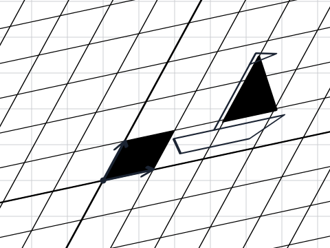
Four numbers in two columns can rotate the plane, stretch it, skew it, reflect it in a mirror or squash it flat onto a line. Let’s learn to read a matrix as the blueprint of a deformation: chain deformations together, undo them, and tell from a single number how much area changes.
 36
Gaussian elimination
How to find a lost planet from a few observations: turn a system of many equations into a staircase and read the answer from the bottom up. The steps show at once whether the system has one solution, infinitely many or none.
 38
Eigenvectors
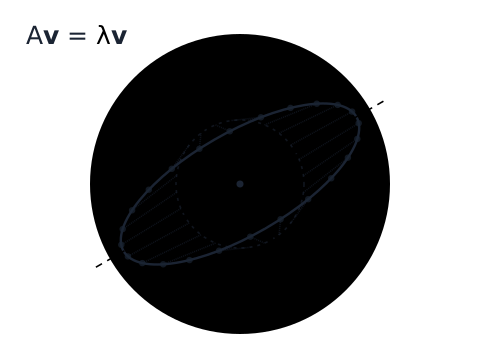
A matrix usually turns vectors, but many matrices have directions they only stretch. Let’s find them, and it will turn out that the Fibonacci numbers, the Google search engine and a tilted ellipse all work the same way.
Other solvers
- Quadratic equation
- Linear equation
- System of linear equations
- Higher-degree equations and factoring
- Inequalities by the interval method
- Derivative
- Integral
- Limit
- Curve sketching
- Fraction arithmetic
- GCD, LCM and Euclid's algorithm
- Prime factorisation
- Solving a triangle
- Trigonometric equation
- Exponential and logarithmic equations
- Percentages, compound interest, loans
- Permutations and combinations
- Number bases
- Complex numbers
- Congruences
- Progressions
- Probability: Bayes and Bernoulli trials
- Differential equation