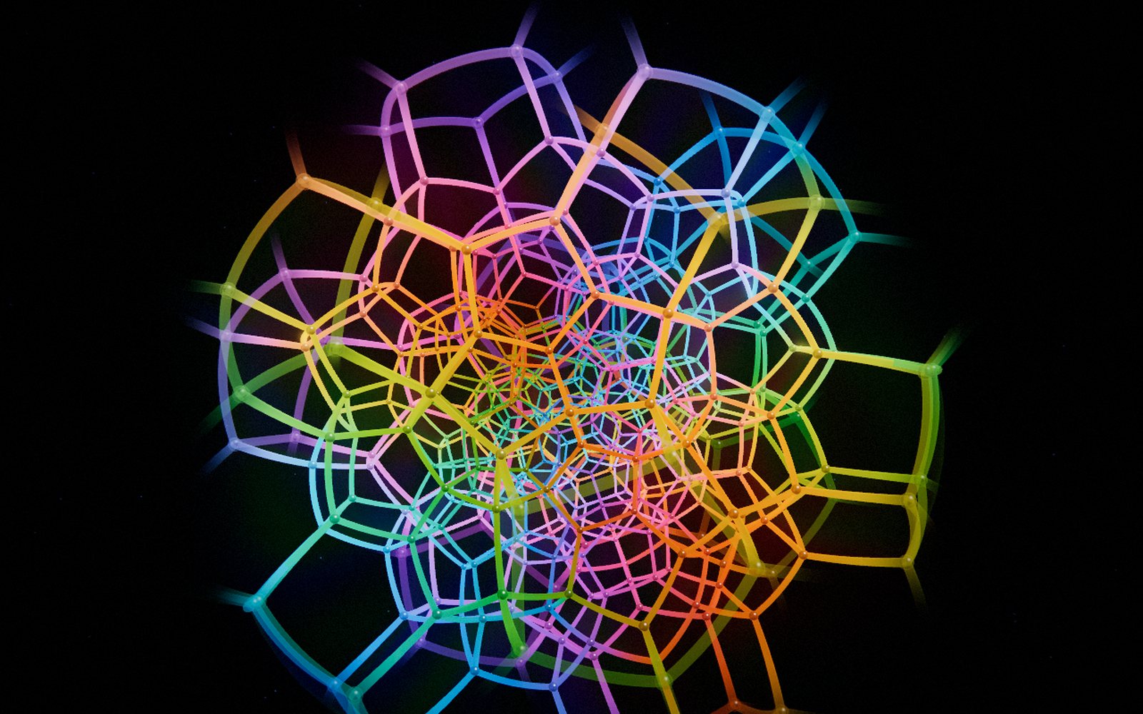
The site has a new section, The Fourth Dimension. It shows live four-dimensional shapes projected into our space, next to an eleven-chapter guide with interactive widgets. The brief was one sentence: build the most advanced and spectacular projection of four-dimensional space into three dimensions, something with a real “wow”. Here is how it works inside: some mathematics, some shaders and an honest list of mistakes.
How do you look into the fourth dimension at all
Edwin Abbott came up with the key trick in 1884, in Flatland. A two-dimensional Square cannot see a three-dimensional sphere, but he can see two things: its shadow on his plane, and its cross-section as the sphere passes through the plane (a point, a growing circle, a shrinking circle, a point again). With four-dimensional shapes we have exactly the same two options: a shadow cast into our space, and a slice cut by our space.
Everything the showcase displays is one or the other. None of it is an artist's impression. The vertices, edges and faces are exact geometry, recomputed from four dimensions into three sixty times a second. You can orbit an ordinary 3D camera, or rotate the object in the fourth dimension: dragging with Shift (or two fingers) pushes the near side of the shape along the fourth dimension in the direction of your gesture.
Building blocks: six regular polytopes from one pipeline
Three dimensions have five regular polyhedra; four dimensions have six: the 5-, 8-, 16-, 24-, 120- and 600-cell. The most complex, the 120-cell, has 600 vertices, 1200 edges, 720 pentagonal faces and 120 dodecahedral cells. Rather than typing all of that into tables, every polytope comes out of one pipeline fed with two lists: the vertices and the normals of the cells.
- A cell is the set of vertices furthest out along its normal.
- A face is where two cells share three or more vertices.
- The edges join neighbouring vertices in each face.
The normals come from the dual polytope: for the tesseract they are the vertices of the 16-cell and vice versa, for the 120-cell they are the vertices of the 600-cell. The 120-cell itself is derived from the 600-cell. The 600-cell's vertices are the 120 “icosians”, quaternions that form a group. The closest pairs give the edges, the sets of four mutually adjacent vertices give 600 tetrahedra, and the centres of those tetrahedra, pushed out to the sphere, are exactly the 600 vertices of the 120-cell. The whole 120-cell is assembled in 7 milliseconds.
On the first run the tests confirmed every count of vertices, edges, faces and cells, and the Euler characteristic V − E + F − C = 0. Only two of my own expectations failed. I thought the central vertex-first section of the tesseract was an octahedron through the midpoints of edges; in fact it passes straight through six vertices, and its volume is 4/3. And using the strings “−0.000000” and “0.000000” as dictionary keys split the Hopf rings in half: 24 rings instead of 12.
One formula for three lenses
We needed at least three projections: an orthographic shadow (the fourth coordinate is simply dropped), a perspective (what is far away in 4D looks smaller), and the stereographic projection (the eye stands on the 3-sphere itself). They turned out to be one formula:
X = (x, y, z) / (1 − k·w)
With k = 0 it is the shadow; with 0 < k < 1 it is a perspective from the point w = 1/k; with k = 1 the eye sits on the pole of the unit sphere, and for points of that sphere this is exactly the stereographic projection. The lens switch on the showcase simply animates k, and the tesseract turns from a “cube inside a cube” into a tangle of arcs right in front of you.
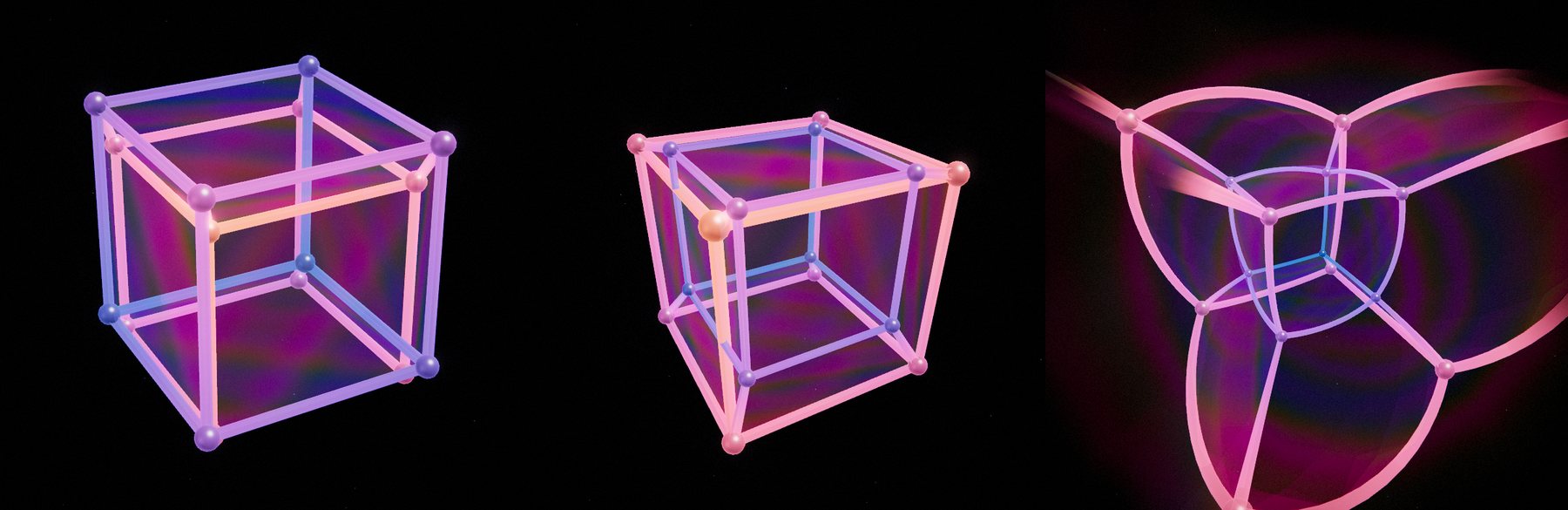
Arched edges and tubes built by the graphics card
In the stereographic projection the edges of a polytope inscribed in the sphere become arcs of circles. The textbook way to get a point on such an arc is slerp, with its sines. There is a simpler way: take the point on the chord and normalise it, p(t) = normalize((1 − t)·a + t·b). The speed along the arc is no longer uniform, but the curve is the same, and in a shader it is one line.
In fact all the four-dimensional maths lives in the vertex shader. The CPU uploads the endpoints of the edges once (two 4D vectors per edge); rotation, projection and building a tube around each edge happen on the GPU, for every vertex, every frame. Each tube is one template cylinder, repeated by instancing. The trickiest part is orienting the tube's cross-section: pick “any perpendicular” and the tube twists. Geometry came to the rescue. With any of our lenses, an edge projects to a segment or an arc of a circle, that is, to a planar curve. The normal of that plane is constant along the whole edge and gives a perfect, twist-free frame.
The second trick is thickness. In the stereographic projection the local scale at a point is 1/(1 − w). Multiply the tube radius by it, and the cells near the projection pole get thick, as they should, while those near the centre get thin. The picture stops looking like wire and gains depth.
Mistakes near the projection pole
The very first frame looked like this:
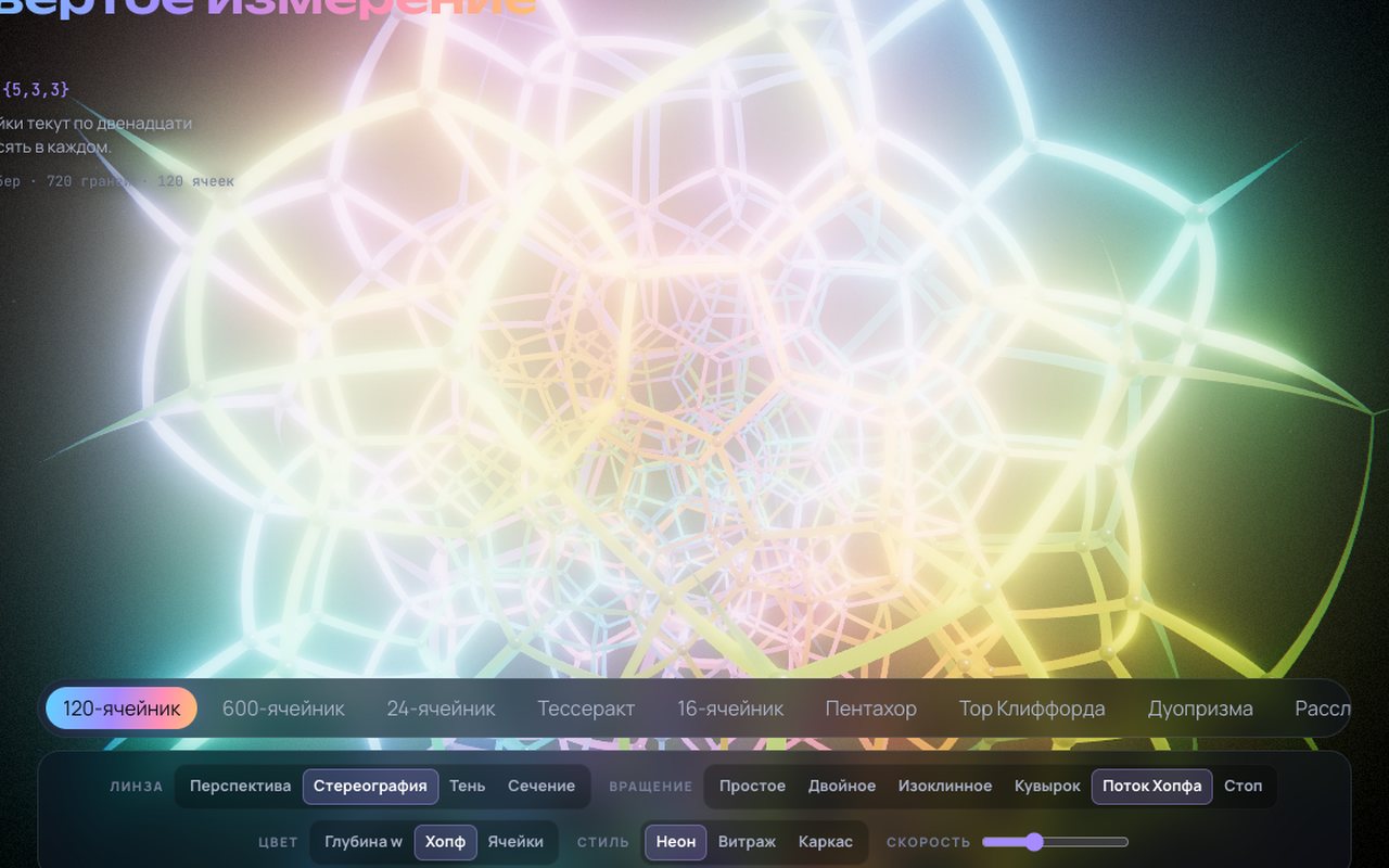
Too much bloom, and translucent faces adding up to white. That is a matter of tuning. The more interesting problem was near the projection pole, where cells swell towards infinity and cover the whole screen. They have to fade out. Attempt one: shrink the tube radius to zero. The result was a sea urchin:
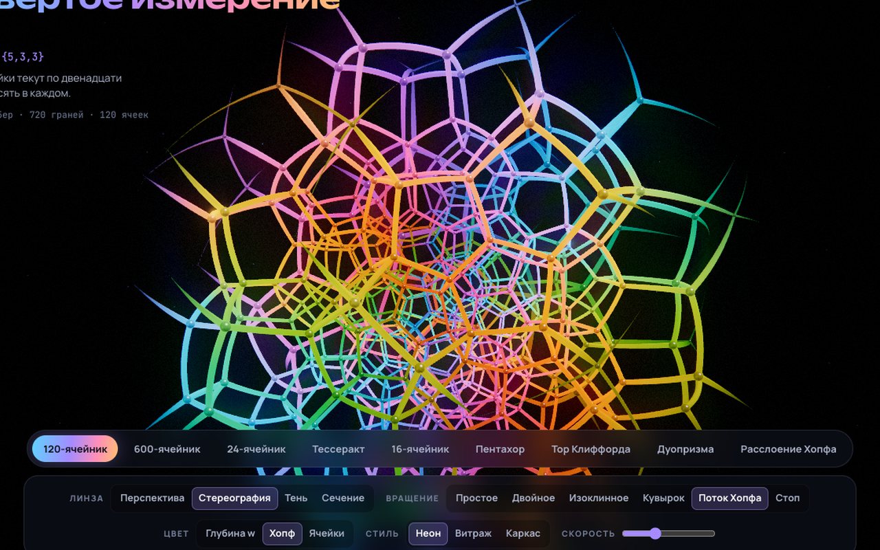
Attempt two was alpha-to-coverage, transparency through the antialiasing samples. It needs no sorting, but with four samples per pixel you see a raster grid instead of a smooth fade. What worked in the end was the most straightforward option: the same geometry is drawn twice, first an opaque pass for everything fully visible, then a blended pass for the fading parts only.
Colour is the fourth coordinate
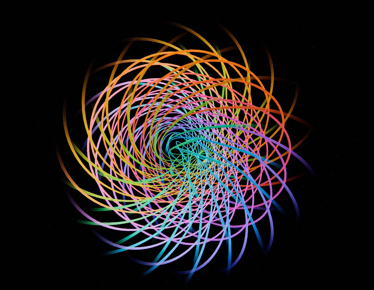
A projection eats one dimension, and colour can at least partly give it back. The “Depth w” palette colours a point by its fourth coordinate: cold blue is farther along the fourth dimension, warm amber is nearer. The colours are built in the perceptual OKLCH space, so the steps look even.
The second palette is “Hopf”. The Hopf map sends a point of the 3-sphere to a point of an ordinary sphere, and all points of one “fibre” (a great circle) get the same colour. The 120-cell has a lovely property here. If the map's axis is taken from a fifth-order quaternion of the same icosian group, its 120 cells fall into exactly 12 rings of 10 dodecahedra, and the 12 image points on the sphere are the vertices of an icosahedron. A test checks this. On the showcase the 120-cell rotates precisely along those rings: the cells flow around twelve circles without changing colour. The Hopf fibration itself is one of the exhibits too: the 3-sphere woven from circles, every two of them linked.
Cross-sections: what a three-dimensional being would see
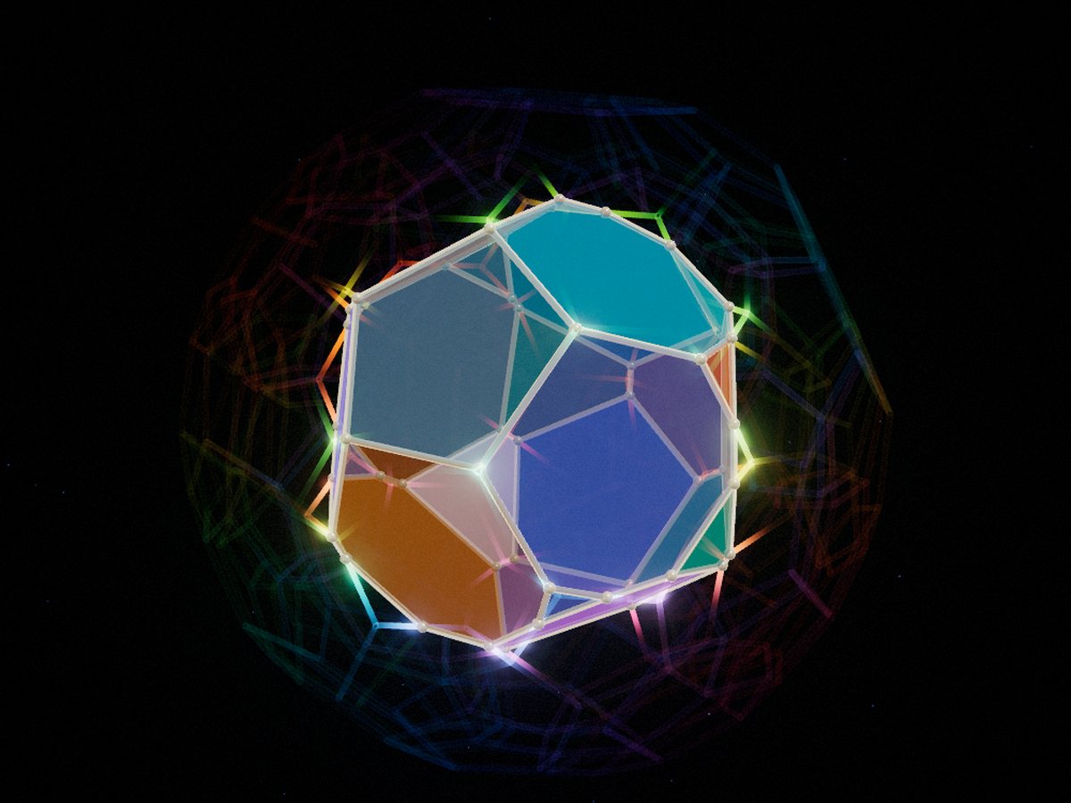
The “Cross-section” lens cuts the shape with the hyperplane w = h and shows what an inhabitant of our space would see as the shape passes through it. For the polytopes the section is recomputed on the CPU every frame. Each cell is a convex 3D solid, its cut by the hyperplane is a convex polygon, and together the polygons bound the section, a polyhedron. The cells get distinct colours (hues a golden angle apart). Behind them the whole shape's shadow glows faintly, and its edges flash where the hyperplane crosses them.
Smooth bodies and a quaternion fractal
Smooth bodies (the hypersphere, the “tiger”, the ditorus, the duocylinder) need no triangles. Their sections are drawn by ray marching. Every body has a four-dimensional distance function. A point X on a ray in our space is lifted into 4D as p = Rᵀ·(X, h), the point of the cutting hyperplane in the body's own coordinates. The key observation: the distance to the body in 4D is never larger than the distance within the slice, because the nearest point in the slice is also somewhere in 4D. So the 4D distance is a safe step for sphere tracing in 3D, and any body with a known distance function can be sliced.
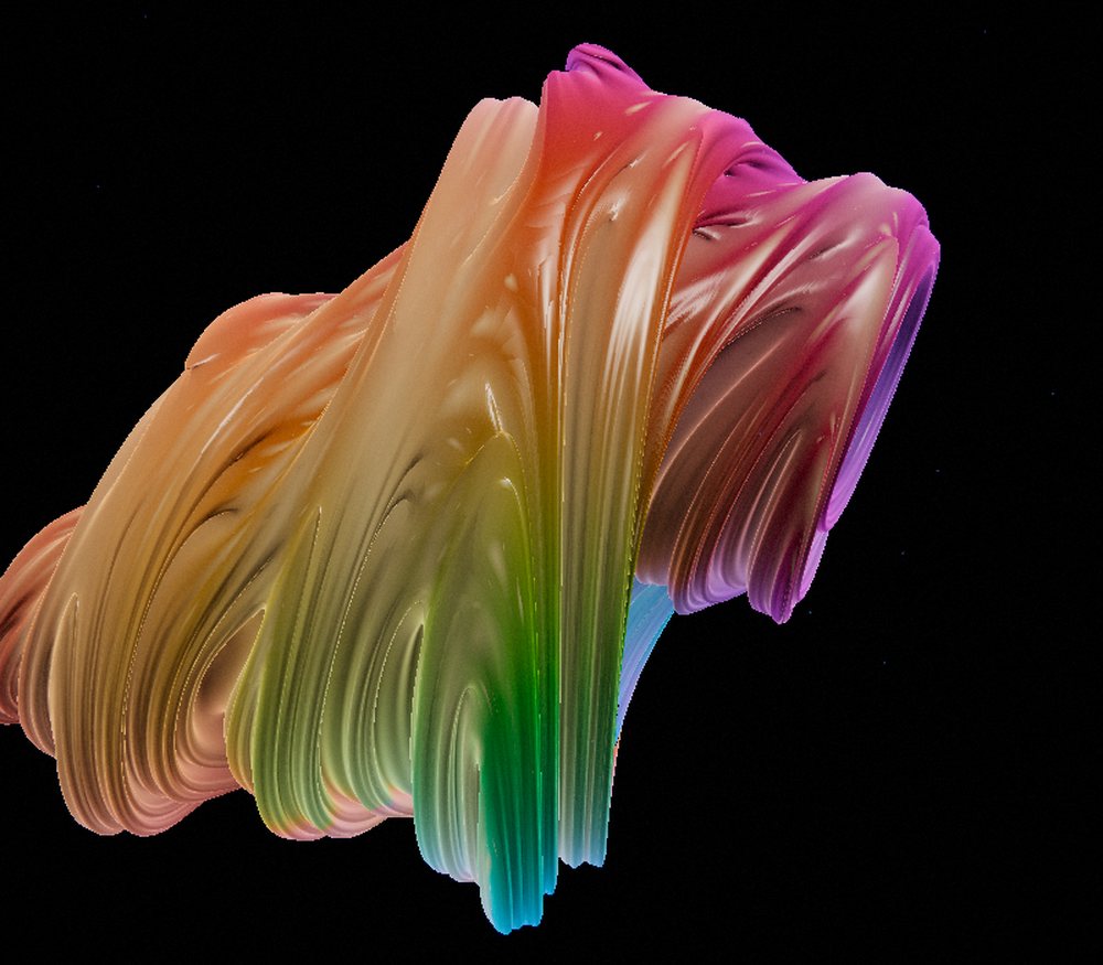
That is where the most unexpected exhibit comes from: the quaternion Julia set. It is the fractal z → z² + c where z and c are quaternions, so the set is four-dimensional. We see its 3D slices while the parameter c slowly drifts around a closed loop, and the fractal keeps flowing into new shapes.
The small things that add up to “wow”
- Film look: HDR rendering, bloom, the ACES tone curve, a light vignette, grain and a barely visible chromatic aberration towards the corners.
- Dust in the background: 900 distant points. As the camera drifts they give parallax, and the eye believes in the depth.
- An entrance: on load, the 120-cell unfolds out of the centre while the camera settles in.
- Speed: the 120-cell is about 440 thousand triangles (1200 tubes, 600 spheres and 720 curved faces). The resolution adapts to the frame rate, and rendering sleeps when the tab is hidden or the scene scrolls away. Headless Chrome on a laptop holds a steady 60 frames per second on all 16 exhibits.
A guide with widgets
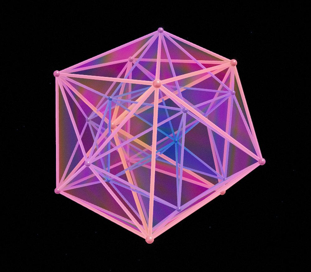
The showcase answers “what does it look like”; the guide answers “why”. It has eleven chapters: what a dimension is, Flatland and thinking by analogy, projections, rotation (in 4D you rotate a plane, not an axis), cross-sections, the six regular polytopes and why there are exactly six, the 3-sphere and the Hopf fibration, the strange geometry of many dimensions (where nearly all of a ball's volume sits right at its surface), where dimensions show up in physics and in data, a history from Schläfli to Interstellar, and a chapter on how the showcase is drawn. The theorems are set apart and proved, and every idea comes with a widget you can play with: extrude a cube into a tesseract, fold Dalí's net, pass a hypersphere through our space.
How the work went
The whole section, from the spec to the deployment, was built by an AI agent: Claude in Claude Code. It first wrote a spec and the maths core with tests, then the showcase. Every change was checked with screenshots from a headless browser: the agent looked at the frames itself and fixed what it saw (all the mistake pictures above come from that loop). Five sub-agents wrote the guide's chapters in parallel from a shared brief covering the markup, the widget API, and the standards for accuracy and sources. The main agent then reviewed their text, formulas and widgets. My part was to set the task, watch and correct. For example, on phones the showcase's header first wrapped onto two lines, and that had to be redone.
Have a look
legost.in/en/utilities/4d. It is best on a big screen. Start with the “Tour”, which walks you through the exhibits and lenses by itself, then move on to the guide.